Inputs and Outputs
After giving a brief command for running ChloroScan, we here explain the inputs and outputs for ChloroScan, and talk about steps in the workflow in more details. We also give some tips for users to check their data and results.
- Overall ChloroScan takes the following inputs:
Metagenomic assembly in fasta format (required): configured by
--Inputs-assemblyDepth profile in tabular format (required
tsv, mutually exclusive with the next): configured by--Inputs-depth-profiledirectory storing alignment in sorted bam format (required): configured by
--Inputs-alignmentBatch name (required, just to distinguish different jobs when running in parallel to avoid overwriting): configured by
--Inputs-batch-name
Commonly for a de novo run we recommend using bam directory, but if you want to rerun your analysis (perhaps adjusting parameters) with present depth profile, you can use it.
The output directory structure of ChloroScan is as follows: (This is a typical example showing only directories)
chloroscan_output
├── logging_info
└── working
    ├── binny
    │   ├── bins
    │   ├── intermediary
    │   │   └── mantis_out
    │   ├── job.errs.outs
    │   ├── logs
    │   └── tmp
    ├── call_contig_depth
    ├── CAT
    ├── cds-extraction
    │   ├── cds
    │   └── faa
    ├── corgi
    ├── FragGeneScanRs
    │   └── GFFs
    ├── refined_bins
    ├── summary
    └── visualizations
Here is a brief description of each step regarding their inputs and outputs.
1. Raw input data
- Metagenomic assembly (.fasta)
ChloroScan takes a metagenomic assembly, which contains all kinds of genomic fragments in the sample including bacteria, archaea, eukaryotes and viruses. The assembly type we currently tested is short-read only, you may derive it from megahit or metaSPAdes. We plan to test the outcome with long reads in the future. Make sure you have contigs with unique ids, and the ids are consistent with the bam files. For example, if your contig id in fasta file is “k141_1000298”, the corresponding contig id in bam file should also be “k141_1000298”. Generally assemblies with on average longer contigs give better results, but it also depends on the quality of assembly.
- Depth profile in BAM format
Through mapping the reads back to the assembly, you can get the depth profile for each contig in samples. For short reads, minimap2 (short read mode), bowtie2 and bwa-mem all works well.
2. Corgi predictions
The input of the first step: contig classification by Corgi requires your input-contigs.fasta only.
The program firstly classifies each contig into five RefSeq-based categories: chloroplast, mitochondria, prokaryote, eukaryote, and unknown.
Then the outputs: classification results: corgi-prediction.csv, and the isolated plastids.fasta file will be generated in the output/working/corgi directory.
The table corgi-prediction.csv contains the contig id, the predicted category, and the posterior probability for each category. The contigs classified as chloroplast with a posterior probability above the specified threshold will be included in the plastids.fasta file.
The table looks like:
file,accession,prediction,probability,original_id,description,Nuclear,Mitochondrion,Plastid,Plasmid,Nuclear/Bacteria,Nuclear/Archaea,Nuclear/Eukaryota,Nuclear/Viruses,Mitochondrion/Eukaryota,Plastid/Eukaryota,Plasmid/Bacteria,Plasmid/Archaea,Plasmid/Eukaryota
assembly.formatted.fa,k97_110,Nuclear/Bacteria,0.5487518906593323,k97_110,k97_110,0.5688353,0.00050010456,0.016087921,0.41457665,0.5487519,0.0055856705,0.006795563,0.007702232,0.0,0.0,0.41455323,2.3394885e-05,4.0987683e-08
assembly.formatted.fa,k97_2859999,Nuclear/Bacteria,0.8199571371078491,k97_2859999,k97_2859999,0.8871814,0.001272265,0.07066683,0.040879533,0.81995714,0.0014582742,0.00072807295,0.06503786,0.0,0.0,0.04087944,9.103693e-08,1.9135307e-09
assembly.formatted.fa,k97_2451439,Plastid,0.8210093379020691,k97_2451439,k97_2451439,0.11955466,0.037155744,0.82100934,0.022280276,0.04770646,0.0004202699,0.04415435,0.027273588,0.0,0.0,0.022280134,1.3834504e-07,2.588508e-09
- To configure this step:
--corgi-pthreshold: the posterior probability threshold to classify a contig into one of the five categories. Default is 0.5.--corgi-min-length: minimum length of contigs to be considered. Default is 1000bp.--corgi-save-filter: run corgi’s default filtering step to isolate plastid contigs, not recommended due to long runtime.--corgi-batch-size: batch size when inferring contigs, default is 1.
3. binning results
The inputs of this step is the plastids.fasta from Corgi and the tabular depth profile with the first column the contig ids and the rest columns the average depths in each sample.
Note: if users did not specify the depth table, ChloroScan directly incorporates the code from binny to generate depth profile. It’s path isoutput/working/depth_profile.txt.
The output directory of binny is in output/working/binny. The directory bins contains the final plastid MAGs in fasta format.
Meanwhile because binny is a snakemake workflow, other intermediary results are also retained in ChloroScan.
Here is a typical example of it:
intermediary
├── annotation_CDS_RNA_hmms_checkm.gff
├── annotation.filt.gff
├── assembly.contig_depth.txt
├── assembly.formatted.fa
├── iteration_1_contigs2clusters.tsv
├── iteration_2_contigs2clusters.tsv
├── iteration_3_contigs2clusters.tsv
├── mantis_out
│   ├── consensus_annotation.tsv
│   ├── integrated_annotation.tsv
│   ├── Mantis.out
│   └── output_annotation.tsv
├── prokka.faa
├── prokka.ffn
├── prokka.fna
├── prokka.fsa
├── prokka.gff
├── prokka.log
├── prokka.tbl
├── prokka.tsv
└── prokka.txt
- To simply, here are the things you need to know:
The input contigs and depth profile in tabular format are in
assembly.formatted.faandassembly.contig_depth.txtrespectively.The predicted open reading frames from contigs are dumped in the file
annotation_CDS_RNA_hmms_checkm.gff.
- To configure this step:
--binning-clustering-hdbscan-min-sample-range: the range of minimum samples parameter when running HDBSCAN clustering, default is 1,5,10.--binning-bin-quality-purity: the minimum purity (i.e. max contamination) threshold for a bin to be retained, default is 90.--binning-bin-quality-min-completeness: the minimum completeness threshold for a bin to be retained, default is 50.--binning-outputdir: the output directory to store binny results before moving it to ChloroScan output, default isoutput/working/binny.--binning-universal-length-cutoff: the length cutoff applied to filter contigs for marker gene prediction and clustering, default is 1500bp.--binning-clustering-epsilon-range: the epsilon range for HDBSCAN. We do not recommend changing this, as it shows minimal effect, default is 0.250,0.000.
For further information on HDBSCAN, see the sklearn docs: https://scikit-learn.org/stable/modules/generated/sklearn.cluster.HDBSCAN.html.
4. CAT
The input is the assembly.formatted.fasta from the intermediary directory. It stores putative plastid contigs longer than 500bp.
Overall the only useful information is in out.CAT.contig2classification.txt, it is a tabular text file storing the classification outcome, putative lineage and the corresponding scores for each taxon for each contig.
It looks like this:
    # contig        classification  reason  lineage lineage scores
k141_1000298        no taxid assigned       no hits to database
k141_1000835        taxid assigned  based on 2/2 ORFs       1;131567;2;1224;28211;54526     1.00;1.00;1.00;1.00;1.00;1.00
k141_1001040        taxid assigned  based on 2/2 ORFs       1;131567;2;1224;28211;766;1699067;2026788       1.00;1.00;1.00;1.00;1.00;1.00;1.00;1.00
k141_1002229        taxid assigned  based on 2/3 ORFs       1;131567;2      1.00;1.00;1.00
...
- To configure this step:
--cat-database: path to CAT database (thedbdirectory), we refer to the directory structure of the most recent CAT db release.--cat-taxonomy: path to the taxonomy file (thetaxonomy/taxdirectory).
5. Summary files
- This step is to summarize the metadata including binning and CAT results. It takes inputs from previous jobs to summarize:
basic information of contigs like GC contents, length, average depths in each sample.
binning results: bin id for each contigs. Unbinned contigs are given as NaN.
CAT results: taxonomic lineage for each contig.
raw sequence.
The output table looks like:
contig id   GC contents     contig depth    contig length   Taxon per Contig        markers on the contig   Contig2Bin      contig sequence
contig_1    0.35    10.5    5000    1;131567;2;1224;28211;54526     atpA,atpB       bin1    ATGCGT...
contig_2    0.40    20.0    3500    1;131567;2;1224;28211;766;1699067;2026788    psaA,psaC,rbcL     bin2    ATGCGT...
contig_3    0.38    15.0    4000    1;131567;2;     rpoC2,rpl4,rpl6 bin3    ATGCGT...
The output summary_table.tsv is a tabular text file storing all the above information for each contig.
5. Refinement module
Though in binning step, binny already takes serious efforts in maintaining the purity of bins. We still found it vulnerable to fragmental contigs by appending them into bins.
So in order to give users a notification, we here reports the contigs with no marker genes predicted by binny and has ambiguous taxonomic classification by CAT (i.e. not eukaryotic or unclassified).
Another way to assist users is to run anvi’o interactive mode to see if contigs form uniform clusters in the phylogram. Further guides: https://astrobiomike.github.io/genomics/metagen_anvio.
The input is the summary_table.tsv from the previous step. The output directory is output/working/refined_bins. We also summarized the information into output/working/refinement_contig_summary.txt to report which contig in which bin has suspicious identity.
6. cds-extraction
For each bin we predict their coding nucleotide sequences and proteins via FragGeneScanRs.
The output is in output/working/cds-extraction. The directory cds contains nucleotide sequences in fna format while faa contains protein sequences in faa format.
- We configure FragGeneScanRs with the following parameters:
-t illumina_5: to use the Illumina error model with 0.5% error rate, which is suitable for metagenomic data.
7. Visualizations
This step generates some visualizations for users to have a glance at their data.
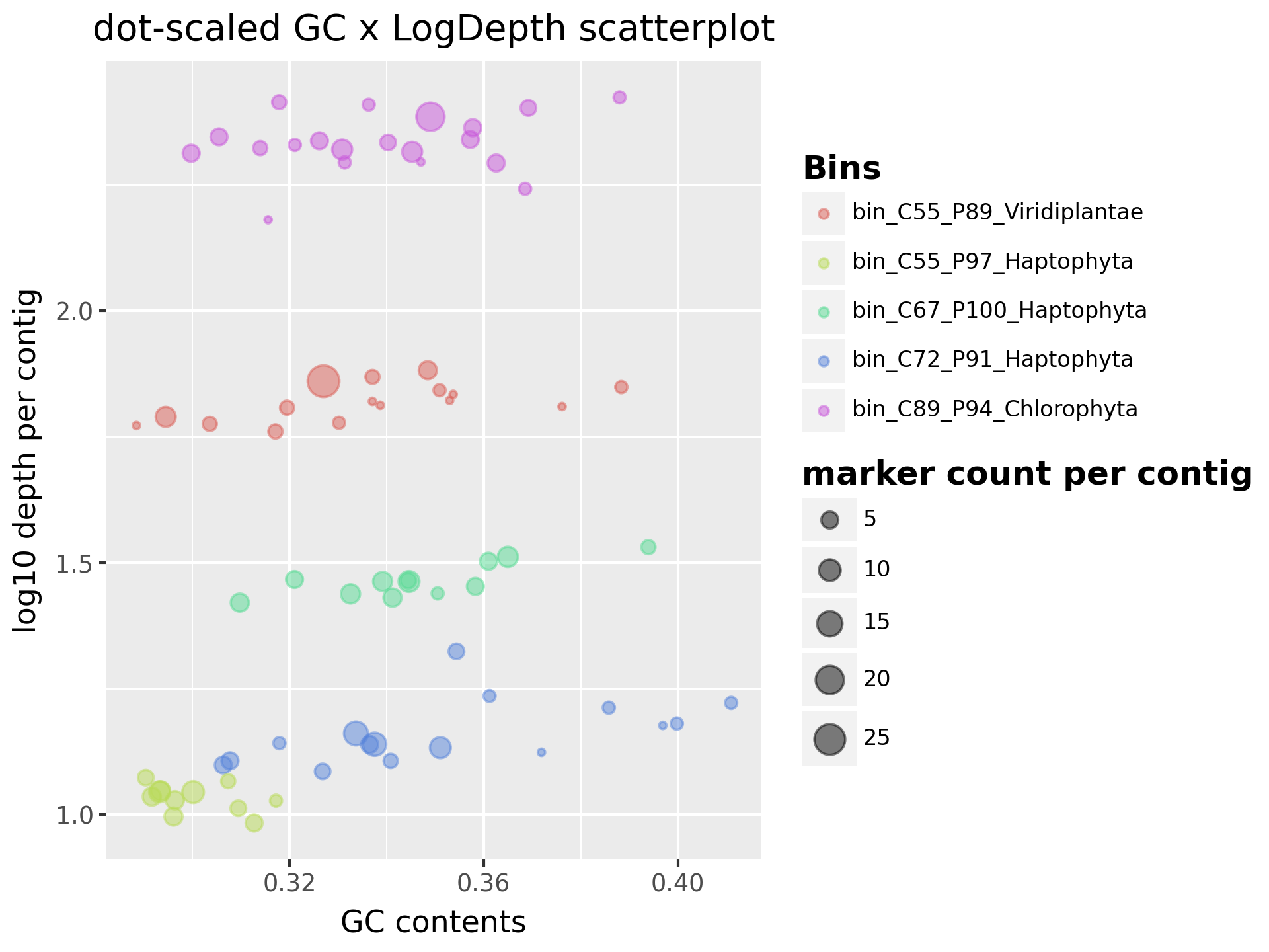
For all MAGs in the sample, we plot their GC contents against their log-transformed pooled average depths. “Pooled” means summing up the depths in each sample for each contig. The output is output/working/visualizations/Scatter_GClogDepth.png.
To differentiate the depths effectively, we applied log transformation to the pooled average depths. As the example shows, the expected good bins should have homogeneous depth and less variable GC contents, thus forming a tight cluster in the plot. On the other hand, bins with more variable depth and GC contents may indicate contamination or misbinning, thus forming a more dispersed cluster in the plot.
- Example:
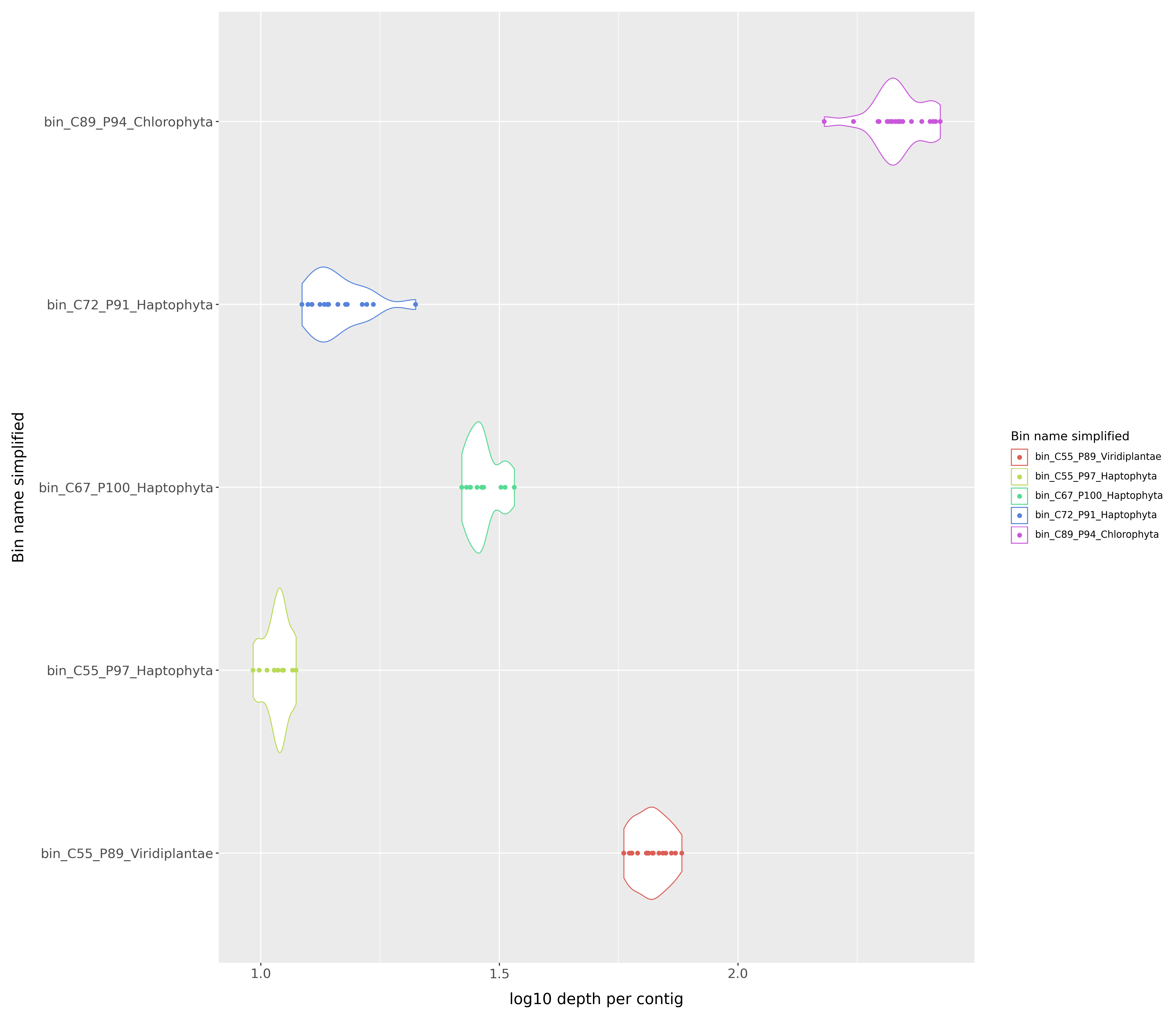
We also generate a violin plot showing the distribution of pooled average depths for all MAGs in the sample. The output is in output/working/visualizations. The file depth_distribution.png is a violin plot showing the distribution of pooled average depths for all MAGs in the sample.
- Example:
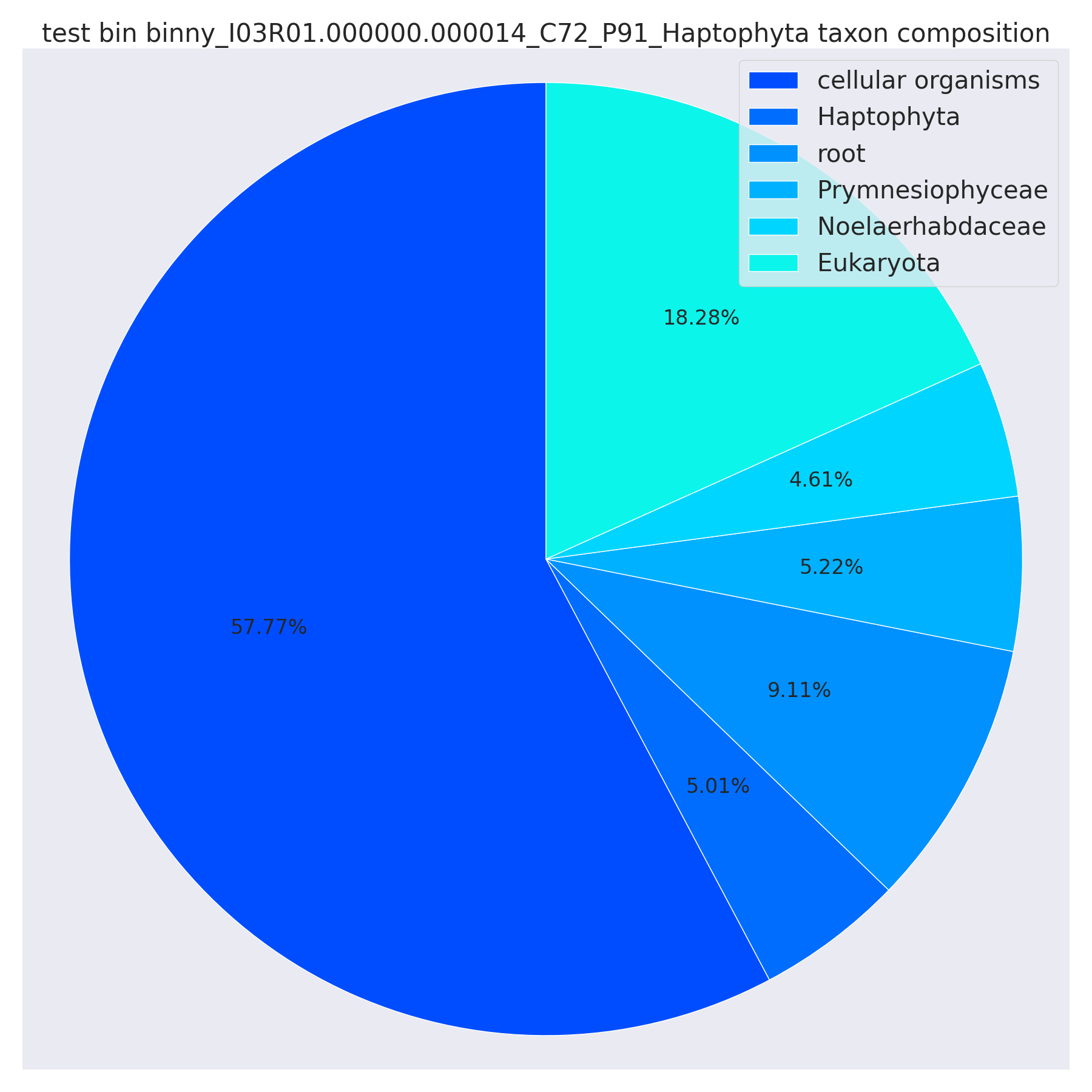
For each bin, we plot their contig-level taxonomy classification (CAT-predicted) in pie charts. The are named as {Batch_name}_{bin_id}_taxonomy_composition.png. Note that CAT may have multiple taxa in a pie chart that roughly points to a taxon of bin (in this case Haptophyte), with some contigs identified at finer level while some were at coarser level. Improved sampling of reference genomes in the future may help.
- Example:
We also prepared a krona plot for the input metagenome, visualizing community-level taxonomy distirbution, the output is Krona.html in the specified output directory. It will show CAT-predicted taxonomy for each putative plastid contig.
- Example:

8. Summary.
- The most important outputs from ChloroScan are listed below:
output/corgi/plastid.fasta, file storing predicted plastid contigs.output/binny/bins, directory storing binny-clustered plastid MAGs in fasta format.output/summary/cross_ref.tsv, a tabular text file storing metadata for each contig including binning and CAT results, as well as raw sequence’s coverage, GC contents.output/visualizations, directory storing plots for users to have a glance at their MAGs for sanity check.output/cds-extraction, the directory stores the predicted ORFs and amino acid sequences, which may work for phylogenetics.